Spelling correction with pyhacrf - Part 2
(Continues from Spelling correction with pyhacrf.)
In this post I’ll look in more detail at how
pyhacrf can
be used to generate spelling corrections for incorrect tokens.
We’ll use cross-validation to set the regularisation
parameter, add character transition features, and compare
the model’s spelling suggestions to a Levenshtein baseline.
Character substitution features
In the previous post I mentioned that one of the advantages that
an HACRF model has above the normal edit distance is that
different character substitutions can have different weights.
That will allow the model to give a higher weight (or probability)
to substituting cat to kat than to hat. I didn’t get around to
showing how it works though.
We have training data like (and about 8000 more examples like this):
x_raw = [('0kkay', 'okay'),
         ('0n', 'on'),
         ('1s', 'once')]
         ('sausge', 'uses'),
         ('finnally', 'mummy'),
         ('bihg', 'morning'),
     ...]
y = ['match', 'match', 'match', 'non-match', 'non-match', ...]
Character substitution feature extraction is added by setting the
transition flag:
fe = StringPairFeatureExtractor(match=True, numeric=True, transition=True)
x = fe.fit_transform(x_raw)
The dimension of the extracted features now jumps from
3 to 3972 (sparse) features.
There are 63 characters in the character set we use here.
If we add a feature for each character to character transition, that
adds 63 x 63 = 3969 features to the 3 that is already there.
The model will learn a parameter for each of these transitions, for
each state (match or non-match at the moment).
For each position in the lattice, if, for example, the character
a occurs in the first string and b in the second string, then
the ('a', 'b') feature will trigger at that position and the
energy of that lattice position will be increased by the
exponent of the corresponding parameter.
Learning
Let’s set the regularisation parameter by doing a parameter sweep.
for i in np.linspace(-8, 4, 15):
    m = Hacrf(l2_regularization=np.exp(i),
              optimizer=fmin_l_bfgs_b,
              optimizer_kwargs={'maxfun': 45})
    x_t, x_v, y_t, y_v = train_test_split(x_train,
                                          y_train,
                                          test_size=0.5)
    m.fit(x_t, y_t)
    train_score = accuracy_score(m.predict(x_t), y_t)
    val_score = accuracy_score(m.predict(x_v), y_v)
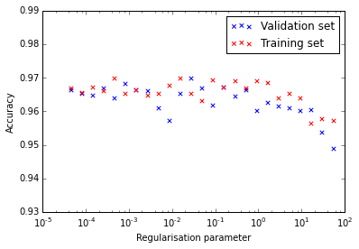
The model that is trained without the transition features have accuracies between 96% and 97% for both the training and testing sets:

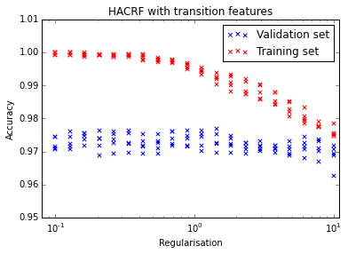
If we add the character transition features, we can see that the model overfits if the regularisation is too low. Initially I thought that 1 looks like a good value, but the transition images below was noisy and a value of 10 made them prettier and more interpretable. In any case the choice of regularisation doesn’t have a huge effect.

The model with character transitions has a 2.4% error on the final test data while the simpler model achieves 2.2% error. Looks like the character transitions don’t add much in this case.
What are the learned weights?
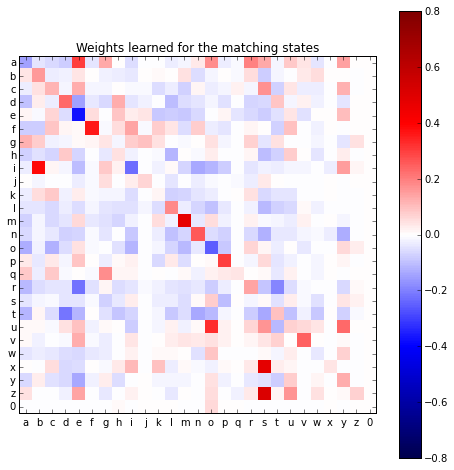
The weights that the model learns for each character transition can be visualised as a character ‘transition matrix’. Let’s just show the first 27 characters, which is the alphabet and ‘0’:
state = 0
plt.imshow(m.parameters[state, 3:].reshape(63, 63)[:27, :27])
state = 1
plt.imshow(m.parameters[state, 3:].reshape(63, 63)[:27, :27])

The first image is the weights corresponding to the 0, or match state.
If the weight is positive then that will make this state more likely and
a negative weight will make the match state less likely.
We can see that the m to m, x to s, z to s, and i to b
transitions are associated with the matching state. It makes sense
that z and s are interchangeable, but i and b doesn’t make sense to me
yet.
0 to o also has a positive weight, which makes sense because there
are examples in the training set such as ('0kkay', 'okay').
Also interesting are the entries on the diagonal—which represents character
matches. I would have guessed that these weights will always be
positive, but all the vowels except u are negative. All the other states’
transition weights have to be taken into account, of course, so it isn’t
as simple as positive weights mean match. If the mismatch states’
weights are even larger negative values then the net effect will still be
to favour the match label.

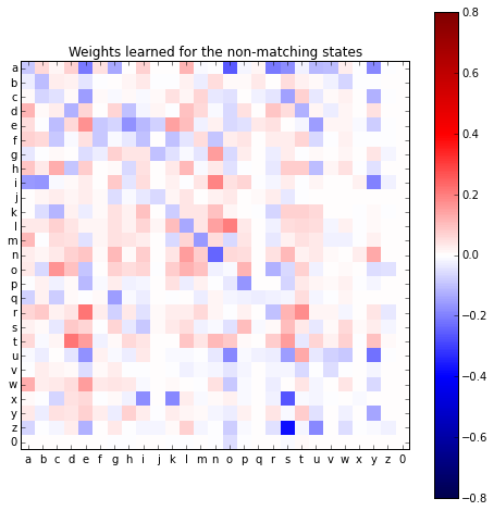
The 1, or non-match state’s weights contain much the same information.
Where there was a positive weight previously there is now a negative weight
and the other way around. One exception is a to a—I can’t think
of a specific reason why this is the case.
Generate candidates
Now let’s evaluate the ranking that the model creates for candidate correct words given incorrectly spelled words.
To do this the 20 000 most common words according to a word frequency
list is used as candidates. The distance (probability of match)
from each of 1 000 incorrect tokens to each of these candidates
is calculated and the 20 000 candidates are sorted according to these
probabilities.
We now check whether the correct (according to our data) word is in the top 1, 3, 20, or 100 candidates.
To speed up the system, the top 1 000 candidates of the Levenshtein baseline (which is much faster than the HACRF) is used as input to the HACRF. The slower model thus only has to score 1 000 candidates per token and not 20 000.
| Method | 1 | 3 | 20 | 100 |
| Levenshtein | 0.47 | 0.61 | 0.74 | 0.82 |
| HACRF without transitions | 0.54 | 0.67 | 0.82 | 0.88 |
| HACRF with transitions | 0.49 | 0.65 | 0.84 | 0.90 |
The HACRF generates better candidates than the baseline, but it seems that adding the transition features unfortunately makes it generate worse candidates.
Conclusion
The addition of the transition features doesn’t improve the performance. This might be because the model is overfitting, and regularisation isn’t really helping.
I only afterwards realised that we have (many) more
parameters than training examples—about 4 000 parameters per state and
transition
(granted that only about 26 x 26 = 729—the alphabet transitions—
are usually triggered).
There are 2 states and 3 transitions per state, which gives about
8 x 4 000 = 32 000 parameters while we have only 6 000 examples—
Always count the parameters!
There are a few things to try:
- Remove the state-transition features. This will immediately bring the total number of parameters down to about 8 000.
- On top of the previous suggestion we can fix the
non-matchparameters to be constant and only train thematchparameters. This will halve the number to about 4 000. - Do some pre-processing or feature selection. Might include something like SVD.
- Try a sparsifying regularisation like L1.
On the one hand I like the idea of throwing all the feature at the model and letting it figure out what works. (CRFs are notoriously used as everything-and-the-kitchen-sink type models)
On the other hand, the traditional and better modeling approach is to rather start with the simplest model and then, by inspecting its output, to increase the complexity where appropriate. I’ll explore some of this in a future post.
See the complete notebook here.
