The package pyugm is a package for learning (discrete at this stage) undirected graphical models in Python. It implements loopy belief propagation (LBP) on cluster graphs or Gibbs sampling for inference. In this post I’ll show how a simple image segmentation model can be build and calibrated.

Interface

The package’s interface is maturing and I think it is almost time to start optimising the run-time. Some of the recent changes are:

• Model objects are now ‘immutable’—the reason I changed this was originally so that we can calculate the factored energy functional, which requires access to the original potentials. But it had the nice benefit that Model objects can be re-used many times.
• All state now lies with Inference objects—much like sklearn. When calibrate is called on an Inference object, Beliefs are updated and afterwards you have an Inference object that represents a calibrated model.
• The calibrate method now takes as parameter the evidence—again I like the parallel to sklearn’s fit method which takes X and y as parameters.

See this notebook for an introduction to the interface.

Anyways let’s get back to the example.

Example problem

As a simple example, let’s say that we have an image that we want to segment into foreground and background. It looks as if very dark and very light pixels are probably foreground and the middle pixel intensities are probably background. (The pixel intensities has been discretized down to 32 possible values.)

Baseline

Let’s first see how good the initial guess is that all those pixel values between 13 and 18 indicate background. We can just directly threshold the pixel values, but let’s rather build it as probabilistic graphical model to illustrate how to do it. Let’s model the problem as a probability model where each pixel-value is a discrete random variable that can take on one of 32 values. Then there is another random variable associated with each pixel that can take on one of 2 values—foreground or background. Let’s call this variable the label.

For the baseline let us suppose that the probability of the image factorize as

\[ p(pixels, labels) = \frac{1}{Z} \prod_{i=0}^{I} \prod_{j=0}^{J} \Psi(pixel_{ij}, label_{ij}), \]

where there are \( I \) rows and \( J \) columns of pixels, and \( Z \) is the normalizing constant. Each \( \Psi \) is a factor that can be represented as a 2 x 32 table with non-negative potentials (one entry for each value that \( label_{ij} \) and \( pixel_{ij} \) can take on).

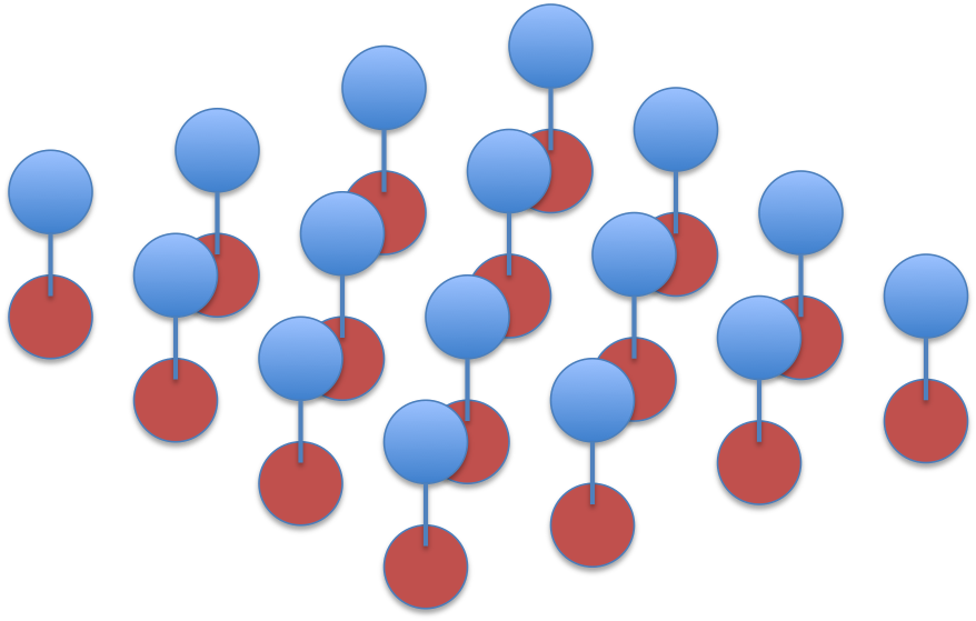
The factorisation is visualised as this graph, where red circles indicate labels and blue circles pixels:

Using pyugm, we create a template for this potential table:

observation_template = np.array([['obs_low'] * 32,
                                 ['obs_high'] * 32])
observation_template[0, 13:17] = 'obs_high'
observation_template[1, 13:17] = 'obs_low'

# Example of a factor using this template
factor = DiscreteFactor([(label_variable_name, 2),
                         (observation_variable_name, 32)],
                        parameters=observation_template))

'obs_low' and 'obs_high' are string placeholders (almost like variables) for the actual floats. It is just convenient to template the values like this so that all the tables (remember there is one table per pixel) can be set to a certain value at once, and to allow us to experiment with different values without having to recreate the model each time.

Now we can loop through each pixel and create its corresponding factor:

I, J = image.shape
factors = []
evidence = {}

for i in xrange(I):
    for j in xrange(J):
        label_variable_name = 'label_{}_{}'.format(i, j)
        observation_variable_name = 'obs_{}_{}'.format(i,j)
        factor = DiscreteFactor([(label_variable_name, 2),
                                 (observation_variable_name, 32)],
                                parameters=observation_template))
        factors.append(factor)
        evidence[observation_variable_name] = image[i, j]

We also add the observation—the actual value that the pixels take on in the image—to the evidence dictionary. Note that each variable must have a name, in this case label_1_5, or obs_9_12 for example. So there are parameter names (obs_low and obs_high) which must be strings, and random variable names (label_2_2 etc) which in our case are strings but can also be ints.

Now we can build the model:

from pyugm.model import Model
model = Model(factors)

Then choose parameters: (let’s choose them so that pixel values between 13 and 18 have a higher background potential than foreground potential—note that we specify the log potentials, hence the negative value for obs_low)

parameters = {'obs_high': 0.1, 'obs_low': -1.0}

And then run inference (doesn’t really do much because the model is just a bunch of disconnected factors):

from pyugm.infer_message import LoopyBeliefUpdateInference
from pyugm.infer_message import FloodingProtocol

order = FloodingProtocol(model, max_iterations=30)
inference = LoopyBeliefUpdateInference(model, order)

inference.calibrate(evidence, parameters)

Now we can visualize the marginal probabilities of each label variable:

labels = np.zeros(image.shape)
for i in xrange(I):
    for j in xrange(J):
        variable_name = 'label_{}_{}'.format(i, j)
        label_factor = inference.get_marginals(variable_name)[0]
        labels[i, j] = label_factor.normalized_data[0] 
plt.imshow(labels, interpolation='nearest')

Black indicates background and white foreground: 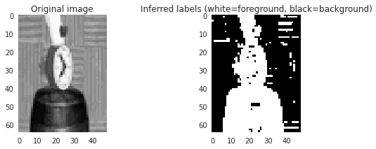So it looks like we are 90% there, it just needs some smoothing out. What we want is a model where background is likely to be surrounded by background and foreground by foreground.

Grid model

To do this let’s relax the assumption that pixel labels are independent. Let’s rather assume that pixel values are independent given the labels, but also that a label is independent of all other labels given its four neighbours:

\[ p(pixels, labels) = \frac{1}{Z} \prod_{i=0}^{I} \prod_{j=0}^{J} \Psi_o(pixel_{ij}, label_{ij}) \Psi_b(label_{ij}, label_{i+1,j})\cdot \\\
\Psi_r(label_{ij}, label_{i,j+1}) \]

(And some special factors on the edges, but let’s leave them out for now.)

The corresponding graph forms a grid:

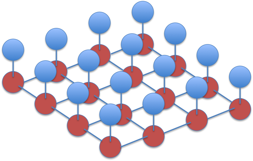
This is a type of Ising grid model. With weak attractive couplings between the labels, loopy belief propagation will probably converge to reasonable marginal beliefs (See for example the paper on Tree reweighted belief propagation).

In addition to the observation_template there is now also the label_template, which introduce two new parameters:

label_template = np.array([['same', 'different'], 
                           ['different', 'same']])

Now we can build the complete grid model:

evidence = {}
factors = []
# Add observation factors
for i in xrange(I):
    for j in xrange(J):
        label_name = 'label_{}_{}'.format(i, j)
        observation_name = 'obs_{}_{}'.format(i, j)
        factor = DiscreteFactor([(label_name, 2),
                                 (observation_name, 32)],
                                parameters=observation_template)
        factors.append(factor)
        evidence[observation_variable_name] = image[i, j]
        
# Add label factors
for i in xrange(I):
    for j in xrange(J):
        variable_name = 'label_{}_{}'.format(i, j)
        if i + 1 < I:
            neighbour_down_name = 'label_{}_{}'.format(i + 1, j)
            factor = DiscreteFactor([(variable_name, 2),
                                     (neighbour_down_name, 2)],
                                    parameters=label_template)
            factors.append(factor)
        if j + 1 < J:
            neighbour_right_name = 'label_{}_{}'.format(i, j + 1)
            factor = DiscreteFactor([(variable_name, 2),
                                     (neighbour_right_name, 2)],
                                    parameters=label_template)
            factors.append(factor)

The calibration of this model is a bit more difficult—it has to run a few iterations. We can peek inside the run by adding a reporter function which records the beliefs of a few random variables and also the belief change and log partition estimate at each iteration:

var_values = {'label_1_1': [],
              'label_10_10': [],
              'label_20_20': [],
              'label_30_30': [],
              'label_40_40': []}
changes = []
partitions = []

# Get some feedback on how inference is converging 
# by listening in on some of the label beliefs.
def reporter(infe, orde):
    # infe: the inference object,
    # orde: the update order object 
    for var in var_values.keys():
        marginal = infe.get_marginals(var)[0].data[0]
        var_values[var].append(marginal)
    change = orde.last_iteration_delta
    changes.append(change)
    energy = infe.partition_approximation()
    partitions.append(energy)
    
model = Model(factors)
order = FloodingProtocol(model, max_iterations=15)
inference = LoopyBeliefUpdateInference(model, 
                                       order,
                                       callback=reporter)

Now let’s choose the parameters so that there is a weak tendency for neighbouring labels to be the same but still a slightly stronger tendency for pixel values between 13 and 17 to be associated with background. (Note that the exact values doesn’t really make that much of a difference—it is fun to play around with them a bit to get a feel for how potentials translate to eventual marginal probabilities though)

Then we run it and plot var_values:

parameters = {'same': 0.1, 'different': -1.0,
              'obs_high': 1.0, 'obs_low': 0.0}
inference.calibrate(evidence, parameters)

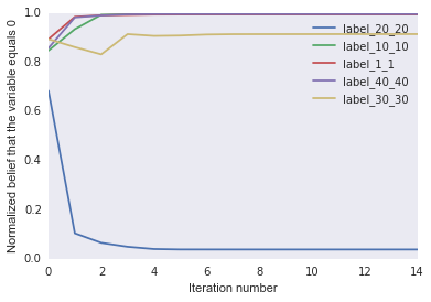
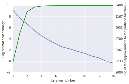
It looks like the label marginals settles down after only a few iterations. The plot of the belief change (blue) and log partition (Z, in green) estimate also show convergence:

Finally let’s visualize the label beliefs:

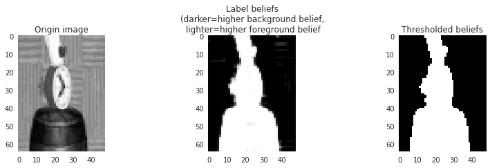
The noise has been smoothed out—and although we know we can’t really trust the beliefs (many went to exactly 1.0 which we know must be impossible for the real marginals), at least they look usable.

See the complete notebook for more detail.