When we want to classify sequences, HCRFs are—if we can forget about recurrent neural networks for a moment—discriminative counterparts to hidden Markov models.

HCRFs for gesture recognition

HCRFs are also called hidden state CRFs, and were introduced as a way to recognise gestures. The assumption is that a gesture is made up out of a sequence of latent poses.

An HMM contains generative models for each of these poses and a transition matrix that describes how the state-sequence evolves. In contrast, an HCRF looks for linear decision boundaries between states and is globally normalised.

The fact that it is globally normalised means that the transition weights cannot be easily interpreted, but (in the un-hidden CRF case at least) this solves the label-bias problem—this problem occurs with maximum entropy models (“halfway” between CRFs and HMMs) and means that state-transitions that don’t occur much in the training data cannot be recognised even with abundant evidence. I’m still figuring out how this works in the hidden CRF case.

pyhcrf package

I toyed around with a Python implementation of HCRFs for my masters project, and eventually put it on Github. It was aimed at sparse text features, was very slow, and could only accept one one-hot encoded word per time-step.

This has now been updated to allow arbitrary features, dense or sparse (depending on whether you pass a numpy ndarray or scipy.sparse.csr_matrix). The inner inference loop is implemented in cython, and everything is wrapped in a sklearn-type interface. (My current favourite interface for these types of projects. The evolution of machine learning interfaces is something that also fascinates me—from sklearn to the dynamic chaining of deep layers in something like caffe or chainer).

Example

Let’s generate some synthetic data to get an intuition for what the model can do. Let’s generate data from two HMMs. There are three states, and each state generates two-dimensional Gaussian output. The model deterministically transitions to the next state after it generates a point.

n_states = 3  
n_dim = 2  # So we can plot samples
states = []
mean = np.array([0, 0])
cov = np.array([[10, 0], 
                [0, 10]])
for state in range(n_states):
        state_mean = np.random.multivariate_normal(mean, cov)
        state_var = np.random.exponential(0.95)
        state_cov = np.array([[state_var, 0],
                              [0, state_var]])
        states.append((state_mean, state_cov))

Now we generate sequences from these states. For the first class we generate sequences that sample from state0 then state1, and then state2, while the second class samples sequences from the reverse. This will (hopefully) demonstrate that the model can differentiate sequences based on the order of points (in contrast to say bag-of-word type models). Sequences can also only include the first two states or the last two states, to show that sequences of different lengths can be handled.

Here are some training examples:

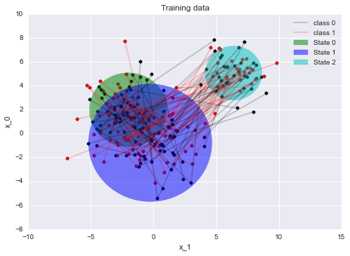
The coloured circles represent one standard deviation of the generating Gaussian distribution.

Now we can train a model:

from sklearn.cross_validation import train_test_split
from sklearn.metrics import confusion_matrix
from pyhcrf import Hcrf

x_train, x_test, y_train, y_test = train_test_split(samples, 
                                                    labels,
                                                    train_size=0.5)
model = Hcrf(num_states=3, 
             l2_regularization=1.0,
             verbosity=10,
             random_seed=3,
             optimizer_kwargs={'maxfun':200})
model.fit(x_train, y_train)
>>        10      -9.17       3.08
>>        20      -9.15       0.08
>>        30      -9.14       1.06
>>        40      -9.11       0.52
>>        50      -9.11       0.19
>>        60      -9.11       0.03
>>        70      -9.11       0.01

pred = model.predict(x_train)
confusion_matrix(y_train, pred)
>> array([[26,  1],
>>        [ 2, 21]])

pred = model.predict(x_test)
confusion_matrix(y_test, pred)
>> array([[21,  2],
>>        [ 2, 25]])

From the confusion matrices it looks like the model can differentiate between the two cases, and it also looks like it generalised to the testing data.

We can visualise the decision surface as a contour plot on the original feature space. Let’s ask the model to classify a sequence where the first element of the sequence coincides with the center of the state1 Gaussian and the second element ranges over the feature space. For each point on the features space we now have the probability that the whole sequence is in class 1 or class 0:

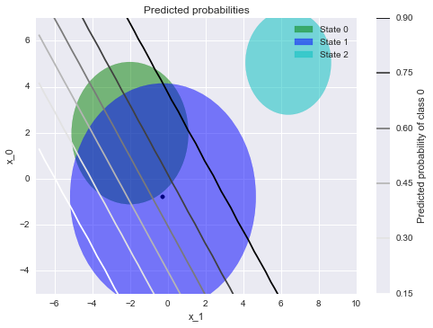
Note that the probability of class 0 is very high if the second point in the sequence were to be near state2. Note also the linear decision boundary and the sigmoidal transition from low to high probability.

Hyper parameters

Let’s investigate how the number of hidden states and the initialisation of the parameters affects the final result for one specific synthetic data set.

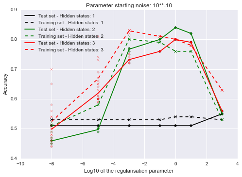
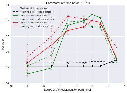
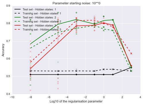
The regularisation parameter has a large effect on the outcome but the amount of noise doesn’t seem to matter that much. The model’s accuracy is sometimes a bit better on the training set because there aren’t many examples, so we just got a few more ‘easy’ points on the testing set.

The fact that both the training and testing accuracies are lower for lower values of the regularisation parameter is puzzling. Usually the training set accuracy is high and the testing accuracy low with low regularisation and the difference decreases as you increase the regularisation.

In this case there might be some numerical issues without regularisation? Or maybe it just gets stuck in a local optima? One way to check it would be to initialise a model with the parameters of a model that was trained with higher regularisation and see whether the accuracy remains high if you then decrease the regularisation parameter. If that is the case then regularisation probably aids optimisation. I’ll check that in a future post.